With Qlik NPrinting, you can present information with the same formatting as in your Qlik application. By default, Qlik NPrinting attempts to preserve the original formats of imported Qlik objects.
When creating templates for generating NPrinting reports, Excel formatting is also available, and you can use this for greater control over the formatting of your reports.
Read on for an example of using Excel conditional formatting to colour cells with a complex conditional formatting requirement.
Complex conditional formatting
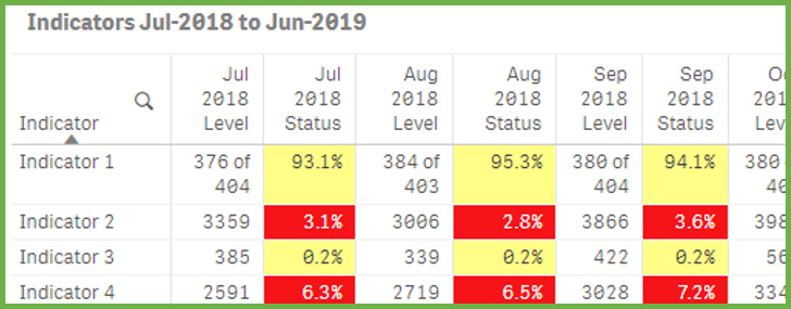
When building a report, I needed to use complex conditional colour formatting on a table. I had created the table in the Qlik application and had applied the formatting to the table.
The table contained indicators, with a level and status for a rolling 12-month period. The status column needed to be coloured based on different criteria for each indicator.
For example, the colour for Indicator 3 should be calculated as follows:
If the numerator is 0 the colour should be green.
If the numerator is between 1- 10 OR the status is less than 5% the colour should be yellow.
Otherwise the colour should be red.

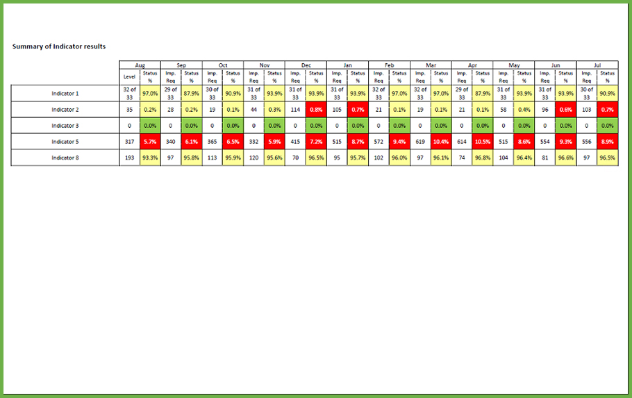
All 25 columns needed to fit on a single A4 size report in landscape orientation.
I initially dragged each column of the straight table into the Excel template, and left the property ‘Keep Source Formats’ for each column ticked. When I previewed the report, the colours that had been calculated and displayed in Qlik were showing correctly. Unfortunately, the width of the columns was too large, causing the table to break over the page in the report.
I was able to get the desired formatting by following these steps:
1.
I added an extra column into the table in Qlik containing the letter representing the calculated colour. (note this object was on a hidden sheet in the Qlik app)
2.
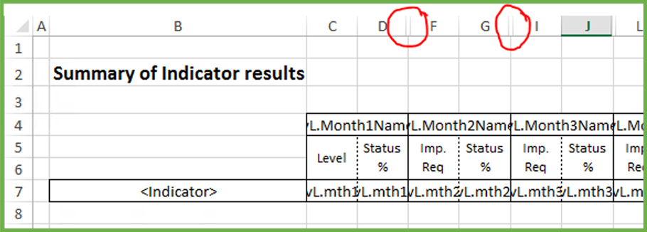
I added the colour column for each month into the NPrinting Excel template, so there were now three columns for each month (Level, Status, Colour).

3.
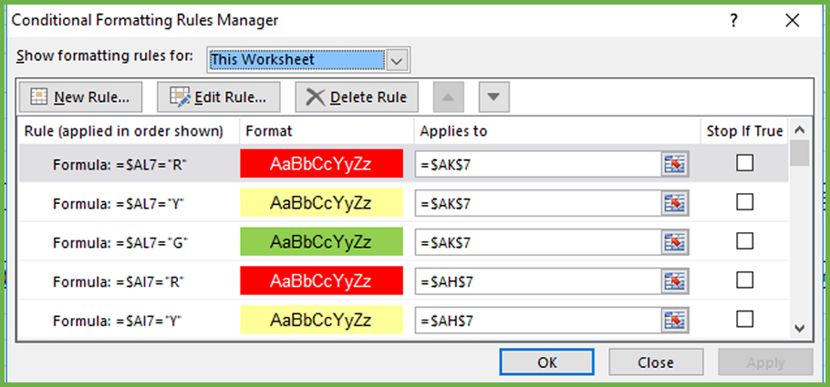
I then added native excel conditional formatting to the status columns, based on the letter in the colour columns.

4.
The colour columns were then hidden in the Excel template and the column widths adjusted so that all columns fitted onto one sheet of A4.

5.
The resulting report was produced in PDF format.

Following these simple steps will help you apply conditional formatting to your NPrinting reports.
Helen Blewett is one of AcumenBI’s specialists in all things Qlik and can help you get the most out NPrinting along with other Qlik applications. If you have questions or would like to discuss this blog then please feel free to contact Helen via email – helenb@acumenbi.co.nz